# Install mlcroissant
!pip install -q mlcroissant h5pyTutorial for GeoCroissant with HDF5 Support 🥐
Introduction

GeoCroissant extends Croissant with geospatial concepts (e.g., spatial extents, coordinate reference systems, temporal coverage), enabling rich, location-aware metadata for Earth-observation and other spatial datasets.
HDF5 Support: This tutorial demonstrates how GeoCroissant works with HDF5 (Hierarchical Data Format 5) files, a powerful format for storing large multi-dimensional arrays commonly used in Earth observation and remote sensing applications. HDF5 offers efficient storage, compression, and fast I/O operations for complex geospatial datasets.
Example: Creating Croissant Metadata for the Landslide4sense Dataset
Let’s try a concrete example with the Landslide4sense dataset hosted on Hugging Face.
This dataset uses HDF5 format to store multi-band satellite imagery and binary landslide masks, making it ideal for demonstrating GeoCroissant’s support for HDF5 files.
import json
from datetime import datetime
# Create a proper GeoCroissant JSON-LD document according to the schema
geocroissant_json = {
"@context": {
"@language": "en",
"@vocab": "https://schema.org/",
"citeAs": "cr:citeAs",
"column": "cr:column",
"conformsTo": "dct:conformsTo",
"cr": "http://mlcommons.org/croissant/",
"geocr": "http://mlcommons.org/croissant/geo/",
"rai": "http://mlcommons.org/croissant/RAI/",
"dct": "http://purl.org/dc/terms/",
"sc": "https://schema.org/",
"data": {
"@id": "cr:data",
"@type": "@json"
},
"examples": {
"@id": "cr:examples",
"@type": "@json"
},
"dataBiases": "cr:dataBiases",
"dataCollection": "cr:dataCollection",
"dataType": {
"@id": "cr:dataType",
"@type": "@vocab"
},
"extract": "cr:extract",
"field": "cr:field",
"fileProperty": "cr:fileProperty",
"fileObject": "cr:fileObject",
"fileSet": "cr:fileSet",
"format": "cr:format",
"includes": "cr:includes",
"isLiveDataset": "cr:isLiveDataset",
"jsonPath": "cr:jsonPath",
"key": "cr:key",
"md5": "cr:md5",
"parentField": "cr:parentField",
"path": "cr:path",
"personalSensitiveInformation": "cr:personalSensitiveInformation",
"recordSet": "cr:recordSet",
"references": "cr:references",
"regex": "cr:regex",
"repeated": "cr:repeated",
"replace": "cr:replace",
"samplingRate": "cr:samplingRate",
"separator": "cr:separator",
"source": "cr:source",
"subField": "cr:subField",
"transform": "cr:transform"
},
"@type": "sc:Dataset",
"name": "Landslide4sense",
"description": "The Landslide4Sense dataset contains satellite imagery for landslide detection, consisting of 3799 training, 245 validation, and 800 test image patches. Each patch is a 128x128 pixel composite of 14 bands including Sentinel-2 multispectral data (B1-B12), slope data, and digital elevation model (DEM) from ALOS PALSAR. All bands are resampled to ~10m resolution and labeled pixel-wise for landslide presence.",
"url": "https://huggingface.co/datasets/ibm-nasa-geospatial/Landslide4sense",
"citeAs": "@dataset{Landslide4sense, title={Landslide4Sense: Reference Benchmark Data and Deep Learning Models for Landslide Detection}, author={Ghorbanzadeh, Omid and Xu, Yongjun and Zhao, Haokun and Wang, Junxi and Zhong, Yanfei and Zhao, Dong and Zang, Qiushi and Wang, Shimin and Zhang, Fang and Shi, Yiliang and others}, year={2022}, url={https://github.com/iarai/Landslide4Sense-2022}}",
"datePublished": "2022-01-01",
"version": "1.0",
"license": "Unknown",
"conformsTo": [
"http://mlcommons.org/croissant/1.1",
"http://mlcommons.org/croissant/geo/1.0"
],
"identifier": "ibm-nasa-geospatial/Landslide4sense",
"alternateName": ["Landslide4Sense-2022", "L4S"],
"creator": {
"@type": "Organization",
"name": "IARAI - Institute for Advanced Research in Artificial Intelligence",
"url": "https://github.com/iarai/Landslide4Sense-2022"
},
"keywords": [
"Landslide4sense",
"landslide detection",
"natural disasters",
"remote sensing",
"satellite imagery",
"Sentinel-2",
"ALOS PALSAR",
"DEM",
"slope",
"geospatial",
"semantic segmentation",
"English",
"1K - 10K",
"Image",
"HDF5",
"Datasets",
"Croissant"
],
"temporalCoverage": "2015-01-01/2022-01-01",
"geocr:coordinateReferenceSystem": "EPSG:4326",
"spatialCoverage": {
"@type": "Place",
"geo": {
"@type": "GeoShape",
"description": "Global coverage with focus on landslide-prone regions"
}
},
"geocr:spatialResolution": {
"@type": "QuantitativeValue",
"value": 10.0,
"unitText": "m"
},
"geocr:samplingStrategy": "Subsetted to 128x128 pixel windows covering landslide and non-landslide areas from global landslide-prone regions",
"geocr:spectralBandMetadata": [
{
"@type": "geocr:SpectralBand",
"name": "B1_Coastal_Aerosol",
"description": "Sentinel-2 Band 1 - Coastal aerosol",
"geocr:centerWavelength": {
"@type": "QuantitativeValue",
"value": 443,
"unitText": "nm"
},
"geocr:bandwidth": {
"@type": "QuantitativeValue",
"value": 20,
"unitText": "nm"
}
},
{
"@type": "geocr:SpectralBand",
"name": "B2_Blue",
"description": "Sentinel-2 Band 2 - Blue",
"geocr:centerWavelength": {
"@type": "QuantitativeValue",
"value": 490,
"unitText": "nm"
},
"geocr:bandwidth": {
"@type": "QuantitativeValue",
"value": 65,
"unitText": "nm"
}
},
{
"@type": "geocr:SpectralBand",
"name": "B3_Green",
"description": "Sentinel-2 Band 3 - Green",
"geocr:centerWavelength": {
"@type": "QuantitativeValue",
"value": 560,
"unitText": "nm"
},
"geocr:bandwidth": {
"@type": "QuantitativeValue",
"value": 35,
"unitText": "nm"
}
},
{
"@type": "geocr:SpectralBand",
"name": "B4_Red",
"description": "Sentinel-2 Band 4 - Red",
"geocr:centerWavelength": {
"@type": "QuantitativeValue",
"value": 665,
"unitText": "nm"
},
"geocr:bandwidth": {
"@type": "QuantitativeValue",
"value": 30,
"unitText": "nm"
}
},
{
"@type": "geocr:SpectralBand",
"name": "B5_Red_Edge_1",
"description": "Sentinel-2 Band 5 - Vegetation Red Edge",
"geocr:centerWavelength": {
"@type": "QuantitativeValue",
"value": 705,
"unitText": "nm"
},
"geocr:bandwidth": {
"@type": "QuantitativeValue",
"value": 15,
"unitText": "nm"
}
},
{
"@type": "geocr:SpectralBand",
"name": "B6_Red_Edge_2",
"description": "Sentinel-2 Band 6 - Vegetation Red Edge",
"geocr:centerWavelength": {
"@type": "QuantitativeValue",
"value": 740,
"unitText": "nm"
},
"geocr:bandwidth": {
"@type": "QuantitativeValue",
"value": 15,
"unitText": "nm"
}
},
{
"@type": "geocr:SpectralBand",
"name": "B7_Red_Edge_3",
"description": "Sentinel-2 Band 7 - Vegetation Red Edge",
"geocr:centerWavelength": {
"@type": "QuantitativeValue",
"value": 783,
"unitText": "nm"
},
"geocr:bandwidth": {
"@type": "QuantitativeValue",
"value": 20,
"unitText": "nm"
}
},
{
"@type": "geocr:SpectralBand",
"name": "B8_NIR",
"description": "Sentinel-2 Band 8 - Near Infrared",
"geocr:centerWavelength": {
"@type": "QuantitativeValue",
"value": 842,
"unitText": "nm"
},
"geocr:bandwidth": {
"@type": "QuantitativeValue",
"value": 115,
"unitText": "nm"
}
},
{
"@type": "geocr:SpectralBand",
"name": "B9_Water_Vapour",
"description": "Sentinel-2 Band 9 - Water vapour",
"geocr:centerWavelength": {
"@type": "QuantitativeValue",
"value": 945,
"unitText": "nm"
},
"geocr:bandwidth": {
"@type": "QuantitativeValue",
"value": 20,
"unitText": "nm"
}
},
{
"@type": "geocr:SpectralBand",
"name": "B10_SWIR_Cirrus",
"description": "Sentinel-2 Band 10 - SWIR - Cirrus",
"geocr:centerWavelength": {
"@type": "QuantitativeValue",
"value": 1375,
"unitText": "nm"
},
"geocr:bandwidth": {
"@type": "QuantitativeValue",
"value": 30,
"unitText": "nm"
}
},
{
"@type": "geocr:SpectralBand",
"name": "B11_SWIR_1",
"description": "Sentinel-2 Band 11 - Short Wave Infrared 1",
"geocr:centerWavelength": {
"@type": "QuantitativeValue",
"value": 1610,
"unitText": "nm"
},
"geocr:bandwidth": {
"@type": "QuantitativeValue",
"value": 90,
"unitText": "nm"
}
},
{
"@type": "geocr:SpectralBand",
"name": "B12_SWIR_2",
"description": "Sentinel-2 Band 12 - Short Wave Infrared 2",
"geocr:centerWavelength": {
"@type": "QuantitativeValue",
"value": 2190,
"unitText": "nm"
},
"geocr:bandwidth": {
"@type": "QuantitativeValue",
"value": 180,
"unitText": "nm"
}
},
{
"@type": "geocr:SpectralBand",
"name": "B13_Slope",
"description": "ALOS PALSAR - Slope data derived from radar",
"dataType": "Topographic"
},
{
"@type": "geocr:SpectralBand",
"name": "B14_DEM",
"description": "ALOS PALSAR - Digital Elevation Model",
"dataType": "Elevation"
}
],
"distribution": [
{
"@type": "cr:FileObject",
"@id": "data_repo",
"name": "data_repo",
"description": "Landslide4sense dataset directory containing HDF5 files",
"contentUrl": "./Landslide4sense",
"encodingFormat": "local_directory",
"sha256": "placeholder_checksum_for_directory"
},
{
"@type": "cr:FileSet",
"@id": "h5-files",
"name": "h5-files",
"description": "All HDF5 files containing images and masks",
"containedIn": {
"@id": "data_repo"
},
"encodingFormat": "application/x-hdf5",
"includes": "**/*.h5"
}
],
"recordSet": [
{
"@type": "cr:RecordSet",
"@id": "landslide4sense",
"name": "landslide4sense",
"description": "Landslide4sense dataset with 14-band satellite imagery and binary mask annotations for landslide detection.",
"field": [
{
"@type": "cr:Field",
"@id": "landslide4sense/image",
"name": "landslide4sense/image",
"description": "File path to HDF5 image file containing 14-band satellite imagery (Sentinel-2 B1-B12, Slope, DEM). Each image is 128x128 pixels with bands stacked as (height, width, bands). Data type: float64. Dataset name within HDF5: 'img'.",
"dataType": "sc:Text",
"source": {
"fileSet": {
"@id": "h5-files"
},
"extract": {
"fileProperty": "fullpath"
},
"transform": {
"regex": "images/.*/image_.*\\.h5$"
}
},
"geocr:bandConfiguration": {
"@type": "geocr:BandConfiguration",
"geocr:totalBands": 14,
"geocr:bandNamesList": [
"B1_Coastal_Aerosol",
"B2_Blue",
"B3_Green",
"B4_Red",
"B5_Red_Edge_1",
"B6_Red_Edge_2",
"B7_Red_Edge_3",
"B8_NIR",
"B9_Water_Vapour",
"B10_SWIR_Cirrus",
"B11_SWIR_1",
"B12_SWIR_2",
"B13_Slope",
"B14_DEM"
]
}
},
{
"@type": "cr:Field",
"@id": "landslide4sense/mask",
"name": "landslide4sense/mask",
"description": "File path to HDF5 mask file containing binary landslide annotations. Each mask is 128x128 pixels with values: 0 (non-landslide) and 1 (landslide). Data type: uint8. Dataset name within HDF5: 'mask'.",
"dataType": "sc:Text",
"source": {
"fileSet": {
"@id": "h5-files"
},
"extract": {
"fileProperty": "fullpath"
},
"transform": {
"regex": "annotations/.*/mask_.*\\.h5$"
}
},
"geocr:bandConfiguration": {
"@type": "geocr:BandConfiguration",
"geocr:totalBands": 1,
"geocr:bandNamesList": ["mask"]
}
},
{
"@type": "cr:Field",
"@id": "landslide4sense/split",
"name": "landslide4sense/split",
"description": "Dataset split indicator extracted from file path (train/validation/test)",
"dataType": "sc:Text",
"source": {
"fileSet": {
"@id": "h5-files"
},
"extract": {
"fileProperty": "fullpath"
},
"transform": {
"regex": "images/(train|validation|test)/"
}
}
}
]
}
]
}
# Write the GeoCroissant JSON-LD to file
with open("landslide4sense_geocroissant.json", "w") as f:
json.dump(geocroissant_json, f, indent=2)When creating Metadata: - We also check for errors in the configuration. - We generate warnings if the configuration doesn’t follow guidelines and best practices.
For instance, in this case:
!mlcroissant validate --jsonld=landslide4sense_geocroissant.jsonI0218 09:01:08.186365 127356445840896 validate.py:53] Done.The validation confirms our GeoCroissant metadata is correctly structured!
Key features of this HDF5-based GeoCroissant metadata:
- Format: HDF5 files (application/x-hdf5)
- Spectral Bands: 14 bands (12 Sentinel-2 + Slope + DEM)
- Spatial Resolution: 10 meters per pixel
- Image Size: 128x128 pixels
- Data Structure:
- Images stored in HDF5 with dataset name ‘img’ (shape: 128, 128, 14)
- Masks stored in HDF5 with dataset name ‘mask’ (shape: 128, 128)
- Band Configuration: Properly defined with
geocr:bandNamesList - Coordinate Reference System: EPSG:4326
Example: Loading the Landslide4sense Dataset
Now that we have our GeoCroissant metadata, we can load the HDF5 dataset files directly.
import h5py
import numpy as np
import matplotlib.pyplot as plt
from pathlib import Path
import json

# Load the GeoCroissant metadata we created
with open("landslide4sense_geocroissant.json", "r") as f:
    metadata = json.load(f)

# Extract key information from metadata
print("Information from GeoCroissant Metadata:")
print(f"  Dataset: {metadata['name']}")
print(f"  Spatial Resolution: {metadata['geocr:spatialResolution']['value']} {metadata['geocr:spatialResolution']['unitText']}")
print(f"  Total Bands: {len(metadata['geocr:spectralBandMetadata'])}")

# Get the dataset path from metadata
dataset_path = Path(metadata['distribution'][0]['contentUrl'])

# Get counts of files in each split
train_images = list((dataset_path / "images" / "train").glob("*.h5"))
val_images = list((dataset_path / "images" / "validation").glob("*.h5"))
test_images = list((dataset_path / "images" / "test").glob("*.h5"))

print(f"\nDataset Structure:")
print(f"  Training: {len(train_images)}, Validation: {len(val_images)}, Test: {len(test_images)}")
print(f"  Total: {len(train_images) + len(val_images) + len(test_images)} samples")
Information from GeoCroissant Metadata:
Dataset: Landslide4sense
Spatial Resolution: 10.0 m
Total Bands: 14
Dataset Structure:
Training: 3799, Validation: 245, Test: 800
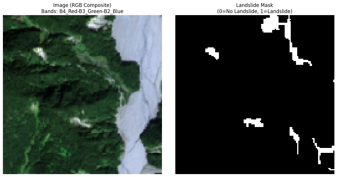
Total: 4844 samplesExample: Visualizing HDF5 Image and Mask from the Landslide4sense Dataset
After inspecting the dataset structure, we load a sample from the training split and visualize both the satellite image and its corresponding landslide mask.
Key steps:
- Retrieve the first sample HDF5 file from the training set
- Read the image data from the ‘img’ dataset (14 bands, 128x128 pixels)
- Read the corresponding mask from the mask HDF5 file
- Create an RGB composite using bands 4, 3, 2 (Red, Green, Blue) from Sentinel-2
- Normalize each RGB channel independently to the
[0,1]range for proper display - Plot the RGB image and the binary landslide mask side-by-side using
matplotlib
# Load metadata to guide data loading
with open("landslide4sense_geocroissant.json", "r") as f:
    metadata = json.load(f)

# Extract band names from metadata
band_names = metadata['recordSet'][0]['field'][0]['geocr:bandConfiguration']['geocr:bandNamesList']

# Find RGB band indices from metadata
rgb_band_names = ['B4_Red', 'B3_Green', 'B2_Blue']
rgb_indices = [band_names.index(band) for band in rgb_band_names]

# Get paths to a sample image and its corresponding mask
if train_images:
    image_file = train_images[0]
    # Extract the image number from filename (e.g., "image_123.h5" -> "123")
    image_number = image_file.stem.split('_')[1]
    mask_file = dataset_path / "annotations" / "train" / f"mask_{image_number}.h5"

    # Read the HDF5 image file (14 bands, 128x128)
    with h5py.File(image_file, 'r') as f:
        image = f['img'][:]  # Shape: (128, 128, 14)

    # Read the HDF5 mask file
    with h5py.File(mask_file, 'r') as f:
        mask = f['mask'][:]  # Shape: (128, 128)

    # Create RGB composite using band indices from metadata
    image_rgb = image[:, :, rgb_indices]  # Extract RGB bands based on metadata

    # Normalize each channel separately for display
    for i in range(3):
        channel = image_rgb[:, :, i]
        min_val = np.min(channel)
        max_val = np.max(channel)
        if max_val > min_val:
            image_rgb[:, :, i] = (channel - min_val) / (max_val - min_val)

    # Plot image and mask side-by-side
    fig, axs = plt.subplots(1, 2, figsize=(12, 6))

    axs[0].imshow(image_rgb)
    axs[0].set_title(f"Image (RGB Composite)\nBands: {'-'.join(rgb_band_names)}", fontsize=12)
    axs[0].axis("off")

    axs[1].imshow(mask, cmap="gray", vmin=0, vmax=1)
    axs[1].set_title("Landslide Mask\n(0=No Landslide, 1=Landslide)", fontsize=12)
    axs[1].axis("off")

    plt.tight_layout()
    plt.show()