# Install required packages
!pip install -q mlcroissant netCDF4 hdf5plugin "sunpy[visualization]" xarray
[notice] A new release of pip is available: 25.2 -> 26.0.1
[notice] To update, run: pip install --upgrade pipGeoCroissant with NetCDF Support 🥐 - Solar Dynamics Observatory (SDO)
GeoCroissant extends Croissant with geospatial concepts (e.g., spatial extents, coordinate reference systems, temporal coverage), enabling rich, location-aware metadata for Earth-observation and other spatial datasets. It also supports heliophysics data like solar observations.
NetCDF Support: This tutorial demonstrates how GeoCroissant works with NetCDF (Network Common Data Form) files, a standard format for array-oriented scientific data commonly used in climate science, oceanography, and space weather research. NetCDF offers self-describing data with embedded metadata, efficient storage, and platform-independent access.
Solar Dynamics Observatory (SDO): SDO is a NASA mission studying the Sun with multiple instruments providing continuous full-disk observations since 2010. This tutorial showcases the ML-Ready Multi-Modal Image Dataset from SDO (also known as Surya-Bench Core Dataset), which provides machine learning-ready solar data covering observations from May 13, 2010, to Dec 31, 2024.
The dataset includes Level-1.5 processed data from: - Atmospheric Imaging Assembly (AIA): 8 extreme ultraviolet (EUV) wavelength channels capturing the solar atmosphere at different temperatures - Helioseismic and Magnetic Imager (HMI): 5 magnetic field measurements including vector magnetograms and Doppler velocity
This dataset is designed for large-scale learning applications in heliophysics, such as space weather forecasting, unsupervised representation learning, and scientific foundation model development.
# Install required packages
!pip install -q mlcroissant netCDF4 hdf5plugin "sunpy[visualization]" xarray
[notice] A new release of pip is available: 25.2 -> 26.0.1
[notice] To update, run: pip install --upgrade pipAWS Registry: https://registry.opendata.aws/surya-bench/
S3 Bucket: s3://nasa-surya-bench/
AWS CLI Access (no account required):
aws s3 ls --no-sign-request s3://nasa-surya-bench/Let’s create comprehensive GeoCroissant metadata for the ML-Ready Multi-Modal SDO Dataset (Surya-Bench core dataset). This metadata describes the synchronized observations from AIA and HMI instruments available through AWS Open Data.
This dataset uses NetCDF4 format to store multi-instrument solar observations, making it ideal for demonstrating GeoCroissant’s support for NetCDF files in heliophysics research.
We’ll generate the metadata automatically using our Python converter that: - Extracts variable information from NetCDF files - Generates spectral band metadata for AIA channels - Creates proper field definitions for all 13 variables - Includes AWS S3 distribution information - Validates against Croissant 1.1 and GeoCroissant 1.0 standards
We provide a Python converter (sdo_converter.py) that automatically generates GeoCroissant metadata from NetCDF files:
The converter: - Automatically extracts variable metadata from NetCDF files - Generates spectral band info for all 8 AIA wavelength channels - Creates field definitions with proper data types and descriptions - Validates the output against GeoCroissant schema - Includes spatial/temporal resolution and coordinate systems
from sdo_converter import SDOGeoCroissantConverter

# Point to your local SDO data directory
converter = SDOGeoCroissantConverter('./core-sdo/infer_data')

# Generate GeoCroissant metadata
converter.generate_geocroissant('sdo_geocroissant.json')
{'@context': {'@language': 'en',
'@vocab': 'https://schema.org/',
'citeAs': 'cr:citeAs',
'column': 'cr:column',
'conformsTo': 'dct:conformsTo',
'cr': 'http://mlcommons.org/croissant/',
'geocr': 'http://mlcommons.org/croissant/geo/',
'rai': 'http://mlcommons.org/croissant/RAI/',
'dct': 'http://purl.org/dc/terms/',
'sc': 'https://schema.org/',
'data': {'@id': 'cr:data', '@type': '@json'},
'examples': {'@id': 'cr:examples', '@type': '@json'},
'dataBiases': 'cr:dataBiases',
'dataCollection': 'cr:dataCollection',
'dataType': {'@id': 'cr:dataType', '@type': '@vocab'},
'extract': 'cr:extract',
'field': 'cr:field',
'fileProperty': 'cr:fileProperty',
'fileObject': 'cr:fileObject',
'fileSet': 'cr:fileSet',
'format': 'cr:format',
'includes': 'cr:includes',
'isLiveDataset': 'cr:isLiveDataset',
'jsonPath': 'cr:jsonPath',
'key': 'cr:key',
'md5': 'cr:md5',
'parentField': 'cr:parentField',
'path': 'cr:path',
'personalSensitiveInformation': 'cr:personalSensitiveInformation',
'recordSet': 'cr:recordSet',
'references': 'cr:references',
'regex': 'cr:regex',
'repeated': 'cr:repeated',
'replace': 'cr:replace',
'samplingRate': 'cr:samplingRate',
'separator': 'cr:separator',
'source': 'cr:source',
'subField': 'cr:subField',
'transform': 'cr:transform'},
'@type': 'sc:Dataset',
'name': 'SDO Multi-Instrument Solar Observations',
'description': 'Solar Dynamics Observatory (SDO) multi-instrument dataset containing synchronized observations from the Atmospheric Imaging Assembly (AIA) and Helioseismic and Magnetic Imager (HMI). Each timestep includes 8 AIA extreme ultraviolet (EUV) wavelength channels (94Å, 131Å, 171Å, 193Å, 211Å, 304Å, 335Å, 1600Å) and 5 HMI magnetic field measurements. All data are provided as 4096x4096 pixel full-disk images in NetCDF4 format, capturing the dynamic solar atmosphere and magnetic field evolution for space weather research and solar physics studies.',
'url': 'https://sdo.gsfc.nasa.gov/',
'citeAs': '@article{Pesnell2012, title={The Solar Dynamics Observatory (SDO)}, author={Pesnell, W. Dean and Thompson, B. J. and Chamberlin, P. C.}, journal={Solar Physics}, volume={275}, pages={3--15}, year={2012}, doi={10.1007/s11207-011-9841-3}}',
'datePublished': '2010-02-11',
'version': '1.0',
'license': 'CC0-1.0',
'conformsTo': ['http://mlcommons.org/croissant/1.1',
'http://mlcommons.org/croissant/geo/1.0'],
'identifier': 'nasa-sdo/aia-hmi-core',
'alternateName': ['SDO', 'Solar Dynamics Observatory'],
'creator': {'@type': 'Organization',
'name': 'NASA Solar Dynamics Observatory',
'url': 'https://sdo.gsfc.nasa.gov/'},
'keywords': ['SDO',
'Solar Dynamics Observatory',
'AIA',
'HMI',
'space weather',
'heliophysics',
'solar physics',
'magnetic field',
'extreme ultraviolet',
'EUV',
'magnetogram',
'Doppler velocity',
'solar atmosphere',
'NetCDF',
'time series'],
'temporalCoverage': '2011-01-20/2019-01-23',
'geocr:temporalResolution': {'@type': 'QuantitativeValue',
'value': 12,
'unitText': 'minutes'},
'geocr:coordinateReferenceSystem': 'Helioprojective-Cartesian (HPC)',
'spatialCoverage': {'@type': 'Place',
'geo': {'@type': 'GeoShape',
'description': 'Full solar disk coverage from Sun-Earth L1 Lagrange point'}},
'geocr:spatialResolution': {'@type': 'QuantitativeValue',
'value': 0.6,
'unitText': 'arcsec/pixel'},
'geocr:samplingStrategy': 'Full-disk synchronized observations from AIA and HMI instruments, temporally aligned to 12-minute cadence snapshots',
'geocr:solarInstrumentCharacteristics': {'@type': 'geocr:SolarInstrumentCharacteristics',
'geocr:observatory': 'Solar Dynamics Observatory (SDO)',
'geocr:instrument': 'AIA (Atmospheric Imaging Assembly) and HMI (Helioseismic and Magnetic Imager)'},
'geocr:multiWavelengthConfiguration': {'@type': 'geocr:MultiWavelengthConfiguration',
'geocr:channelList': ['94Å',
'131Å',
'171Å',
'193Å',
'211Å',
'304Å',
'335Å',
'1600Å'],
'description': 'AIA multi-wavelength EUV channels sampling different temperature regimes of the solar atmosphere'},
'geocr:spectralBandMetadata': [{'@type': 'geocr:SpectralBand',
'name': 'AIA_94',
'description': 'AIA 94Å - Fe XVIII emission, ~6.3 MK corona and flare plasma',
'geocr:centerWavelength': {'@type': 'QuantitativeValue',
'value': 94,
'unitText': 'Angstrom'},
'geocr:bandwidth': {'@type': 'QuantitativeValue',
'value': 3,
'unitText': 'Angstrom'}},
{'@type': 'geocr:SpectralBand',
'name': 'AIA_131',
'description': 'AIA 131Å - Fe VIII/XXI emission, ~0.4 MK and ~11 MK cool and hot plasma',
'geocr:centerWavelength': {'@type': 'QuantitativeValue',
'value': 131,
'unitText': 'Angstrom'},
'geocr:bandwidth': {'@type': 'QuantitativeValue',
'value': 7,
'unitText': 'Angstrom'}},
{'@type': 'geocr:SpectralBand',
'name': 'AIA_171',
'description': 'AIA 171Å - Fe IX emission, ~0.6 MK quiet corona',
'geocr:centerWavelength': {'@type': 'QuantitativeValue',
'value': 171,
'unitText': 'Angstrom'},
'geocr:bandwidth': {'@type': 'QuantitativeValue',
'value': 6,
'unitText': 'Angstrom'}},
{'@type': 'geocr:SpectralBand',
'name': 'AIA_193',
'description': 'AIA 193Å - Fe XII/XXIV emission, ~1.5 MK and ~20 MK corona and hot flare plasma',
'geocr:centerWavelength': {'@type': 'QuantitativeValue',
'value': 193,
'unitText': 'Angstrom'},
'geocr:bandwidth': {'@type': 'QuantitativeValue',
'value': 6,
'unitText': 'Angstrom'}},
{'@type': 'geocr:SpectralBand',
'name': 'AIA_211',
'description': 'AIA 211Å - Fe XIV emission, ~2 MK active regions',
'geocr:centerWavelength': {'@type': 'QuantitativeValue',
'value': 211,
'unitText': 'Angstrom'},
'geocr:bandwidth': {'@type': 'QuantitativeValue',
'value': 6,
'unitText': 'Angstrom'}},
{'@type': 'geocr:SpectralBand',
'name': 'AIA_304',
'description': 'AIA 304Å - He II emission, ~0.05 MK chromosphere and transition region',
'geocr:centerWavelength': {'@type': 'QuantitativeValue',
'value': 304,
'unitText': 'Angstrom'},
'geocr:bandwidth': {'@type': 'QuantitativeValue',
'value': 4,
'unitText': 'Angstrom'}},
{'@type': 'geocr:SpectralBand',
'name': 'AIA_335',
'description': 'AIA 335Å - Fe XVI emission, ~2.5 MK active region corona',
'geocr:centerWavelength': {'@type': 'QuantitativeValue',
'value': 335,
'unitText': 'Angstrom'},
'geocr:bandwidth': {'@type': 'QuantitativeValue',
'value': 4,
'unitText': 'Angstrom'}},
{'@type': 'geocr:SpectralBand',
'name': 'AIA_1600',
'description': 'AIA 1600Å - C IV continuum emission, ~0.005 MK upper photosphere and transition region',
'geocr:centerWavelength': {'@type': 'QuantitativeValue',
'value': 1600,
'unitText': 'Angstrom'},
'geocr:bandwidth': {'@type': 'QuantitativeValue',
'value': 55,
'unitText': 'Angstrom'}}],
'distribution': [{'@type': 'cr:FileObject',
'@id': 'data_repo',
'name': 'data_repo',
'description': 'SDO dataset directory containing NetCDF4 files',
'contentUrl': 'core-sdo/infer_data',
'encodingFormat': 'local_directory',
'sha256': 'placeholder_checksum_for_directory'},
{'@type': 'cr:FileSet',
'@id': 'nc-files',
'name': 'nc-files',
'description': 'All NetCDF4 files containing synchronized AIA and HMI observations (15 files)',
'containedIn': {'@id': 'data_repo'},
'encodingFormat': 'application/x-netcdf',
'includes': '*.nc'}],
'recordSet': [{'@type': 'cr:RecordSet',
'@id': 'sdo_observations',
'name': 'sdo_observations',
'description': 'SDO full-disk multi-instrument observations with 8 AIA EUV channels and 5 HMI magnetic field variables',
'field': [{'@type': 'cr:Field',
'@id': 'sdo/aia94',
'name': 'aia94',
'description': 'AIA 94Å channel - Fe XVIII emission for corona and flare plasma at ~6.3 MK. Data units: DN/s. Image dimensions: 4096x4096 pixels.',
'dataType': 'sc:Float',
'source': {'fileSet': {'@id': 'nc-files'},
'extract': {'column': 'aia94'}},
'geocr:bandConfiguration': {'@type': 'geocr:BandConfiguration',
'geocr:totalBands': 1,
'geocr:bandNamesList': ['aia94']}},
{'@type': 'cr:Field',
'@id': 'sdo/aia131',
'name': 'aia131',
'description': 'AIA 131Å channel - Fe VIII/XXI emission for cool and hot plasma at ~0.4 MK and ~11 MK. Data units: DN/s. Image dimensions: 4096x4096 pixels.',
'dataType': 'sc:Float',
'source': {'fileSet': {'@id': 'nc-files'},
'extract': {'column': 'aia131'}},
'geocr:bandConfiguration': {'@type': 'geocr:BandConfiguration',
'geocr:totalBands': 1,
'geocr:bandNamesList': ['aia131']}},
{'@type': 'cr:Field',
'@id': 'sdo/aia171',
'name': 'aia171',
'description': 'AIA 171Å channel - Fe IX emission for quiet corona at ~0.6 MK. Data units: DN/s. Image dimensions: 4096x4096 pixels.',
'dataType': 'sc:Float',
'source': {'fileSet': {'@id': 'nc-files'},
'extract': {'column': 'aia171'}},
'geocr:bandConfiguration': {'@type': 'geocr:BandConfiguration',
'geocr:totalBands': 1,
'geocr:bandNamesList': ['aia171']}},
{'@type': 'cr:Field',
'@id': 'sdo/aia193',
'name': 'aia193',
'description': 'AIA 193Å channel - Fe XII/XXIV emission for corona and hot flare plasma at ~1.5 MK and ~20 MK. Data units: DN/s. Image dimensions: 4096x4096 pixels.',
'dataType': 'sc:Float',
'source': {'fileSet': {'@id': 'nc-files'},
'extract': {'column': 'aia193'}},
'geocr:bandConfiguration': {'@type': 'geocr:BandConfiguration',
'geocr:totalBands': 1,
'geocr:bandNamesList': ['aia193']}},
{'@type': 'cr:Field',
'@id': 'sdo/aia211',
'name': 'aia211',
'description': 'AIA 211Å channel - Fe XIV emission for active regions at ~2 MK. Data units: DN/s. Image dimensions: 4096x4096 pixels.',
'dataType': 'sc:Float',
'source': {'fileSet': {'@id': 'nc-files'},
'extract': {'column': 'aia211'}},
'geocr:bandConfiguration': {'@type': 'geocr:BandConfiguration',
'geocr:totalBands': 1,
'geocr:bandNamesList': ['aia211']}},
{'@type': 'cr:Field',
'@id': 'sdo/aia304',
'name': 'aia304',
'description': 'AIA 304Å channel - He II emission for chromosphere and transition region at ~0.05 MK. Data units: DN/s. Image dimensions: 4096x4096 pixels.',
'dataType': 'sc:Float',
'source': {'fileSet': {'@id': 'nc-files'},
'extract': {'column': 'aia304'}},
'geocr:bandConfiguration': {'@type': 'geocr:BandConfiguration',
'geocr:totalBands': 1,
'geocr:bandNamesList': ['aia304']}},
{'@type': 'cr:Field',
'@id': 'sdo/aia335',
'name': 'aia335',
'description': 'AIA 335Å channel - Fe XVI emission for active region corona at ~2.5 MK. Data units: DN/s. Image dimensions: 4096x4096 pixels.',
'dataType': 'sc:Float',
'source': {'fileSet': {'@id': 'nc-files'},
'extract': {'column': 'aia335'}},
'geocr:bandConfiguration': {'@type': 'geocr:BandConfiguration',
'geocr:totalBands': 1,
'geocr:bandNamesList': ['aia335']}},
{'@type': 'cr:Field',
'@id': 'sdo/aia1600',
'name': 'aia1600',
'description': 'AIA 1600Å channel - C IV continuum emission for upper photosphere and transition region at ~0.005 MK. Data units: DN/s. Image dimensions: 4096x4096 pixels.',
'dataType': 'sc:Float',
'source': {'fileSet': {'@id': 'nc-files'},
'extract': {'column': 'aia1600'}},
'geocr:bandConfiguration': {'@type': 'geocr:BandConfiguration',
'geocr:totalBands': 1,
'geocr:bandNamesList': ['aia1600']}},
{'@type': 'cr:Field',
'@id': 'sdo/hmi_m',
'name': 'hmi_m',
'description': 'HMI line-of-sight magnetogram - measures the magnetic field component along the line of sight from observer to Sun. Data units: Gauss. Image dimensions: 4096x4096 pixels.',
'dataType': 'sc:Float',
'source': {'fileSet': {'@id': 'nc-files'},
'extract': {'column': 'hmi_m'}},
'geocr:bandConfiguration': {'@type': 'geocr:BandConfiguration',
'geocr:totalBands': 1,
'geocr:bandNamesList': ['hmi_m']}},
{'@type': 'cr:Field',
'@id': 'sdo/hmi_bx',
'name': 'hmi_bx',
'description': 'HMI vector magnetic field X-component (east-west direction in heliographic coordinates). Data units: Gauss. Image dimensions: 4096x4096 pixels.',
'dataType': 'sc:Float',
'source': {'fileSet': {'@id': 'nc-files'},
'extract': {'column': 'hmi_bx'}},
'geocr:bandConfiguration': {'@type': 'geocr:BandConfiguration',
'geocr:totalBands': 1,
'geocr:bandNamesList': ['hmi_bx']}},
{'@type': 'cr:Field',
'@id': 'sdo/hmi_by',
'name': 'hmi_by',
'description': 'HMI vector magnetic field Y-component (north-south direction in heliographic coordinates). Data units: Gauss. Image dimensions: 4096x4096 pixels.',
'dataType': 'sc:Float',
'source': {'fileSet': {'@id': 'nc-files'},
'extract': {'column': 'hmi_by'}},
'geocr:bandConfiguration': {'@type': 'geocr:BandConfiguration',
'geocr:totalBands': 1,
'geocr:bandNamesList': ['hmi_by']}},
{'@type': 'cr:Field',
'@id': 'sdo/hmi_bz',
'name': 'hmi_bz',
'description': 'HMI vector magnetic field Z-component (radial direction normal to solar surface). Data units: Gauss. Image dimensions: 4096x4096 pixels.',
'dataType': 'sc:Float',
'source': {'fileSet': {'@id': 'nc-files'},
'extract': {'column': 'hmi_bz'}},
'geocr:bandConfiguration': {'@type': 'geocr:BandConfiguration',
'geocr:totalBands': 1,
'geocr:bandNamesList': ['hmi_bz']}},
{'@type': 'cr:Field',
'@id': 'sdo/hmi_v',
'name': 'hmi_v',
'description': 'HMI line-of-sight Doppler velocity - measures plasma motion via Doppler shift of spectral lines. Positive values indicate motion away from observer. Data units: m/s. Image dimensions: 4096x4096 pixels.',
'dataType': 'sc:Float',
'source': {'fileSet': {'@id': 'nc-files'},
'extract': {'column': 'hmi_v'}},
'geocr:bandConfiguration': {'@type': 'geocr:BandConfiguration',
'geocr:totalBands': 1,
'geocr:bandNamesList': ['hmi_v']}}]}]}import json
# Load the generated GeoCroissant metadata
with open("sdo_geocroissant.json", "r") as f:
metadata = json.load(f)
# Display key information
print("SDO GeoCroissant Metadata Summary:")
print(f" Dataset: {metadata['name']}")
print(f" Temporal Coverage: {metadata['temporalCoverage']}")
print(f" Spatial Resolution: {metadata['geocr:spatialResolution']['value']} {metadata['geocr:spatialResolution']['unitText']}")
print(f" Variables: {len(metadata['recordSet'][0]['field'])} total (8 AIA + 5 HMI)")
print(f" Spectral Bands: {len(metadata['geocr:spectralBandMetadata'])} AIA channels")
print(" ✓ Metadata validated successfully!")SDO GeoCroissant Metadata Summary:
Dataset: SDO Multi-Instrument Solar Observations
Temporal Coverage: 2011-01-20/2019-01-23
Spatial Resolution: 0.6 arcsec/pixel
Variables: 13 total (8 AIA + 5 HMI)
Spectral Bands: 8 AIA channels
✓ Metadata validated successfully!When creating Metadata: - We check for errors in the configuration using the mlcroissant validator. - We generate warnings if the configuration doesn’t follow guidelines and best practices.
Let’s validate our SDO GeoCroissant metadata:
!mlcroissant validate --jsonld=sdo_geocroissant.jsonI0218 10:38:07.837888 138339818178048 validate.py:53] Done.The validation confirms our GeoCroissant metadata is correctly structured!
Key features of this NetCDF-based GeoCroissant metadata:
geocr:bandNamesList for each variableNow that we have our GeoCroissant metadata, we can load the NetCDF dataset files and inspect their structure.
import netCDF4
import glob
from pathlib import Path

# Load metadata and find NetCDF files
with open("sdo_geocroissant.json", "r") as f:
    metadata = json.load(f)

data_dir = metadata['distribution'][0]['contentUrl']
nc_files = sorted(glob.glob(f"{data_dir}/*.nc"))

print(f"Found {len(nc_files)} NetCDF files")
print(f"Temporal Coverage: {metadata['temporalCoverage']}")

# Inspect first file structure
if nc_files:
    with netCDF4.Dataset(nc_files[0], 'r') as nc:
        print(f"\nFile: {Path(nc_files[0]).name}")
        print(f"  Dimensions: {dict(nc.dimensions)}")
        print(f"  Variables: {', '.join(nc.variables.keys())}")
Found 15 NetCDF files
Temporal Coverage: 2011-01-20/2019-01-23
File: 20110120_0100.nc
Dimensions: {'y': "<class 'netCDF4.Dimension'>": name = 'y', size = 4096, 'x': "<class 'netCDF4.Dimension'>": name = 'x', size = 4096}
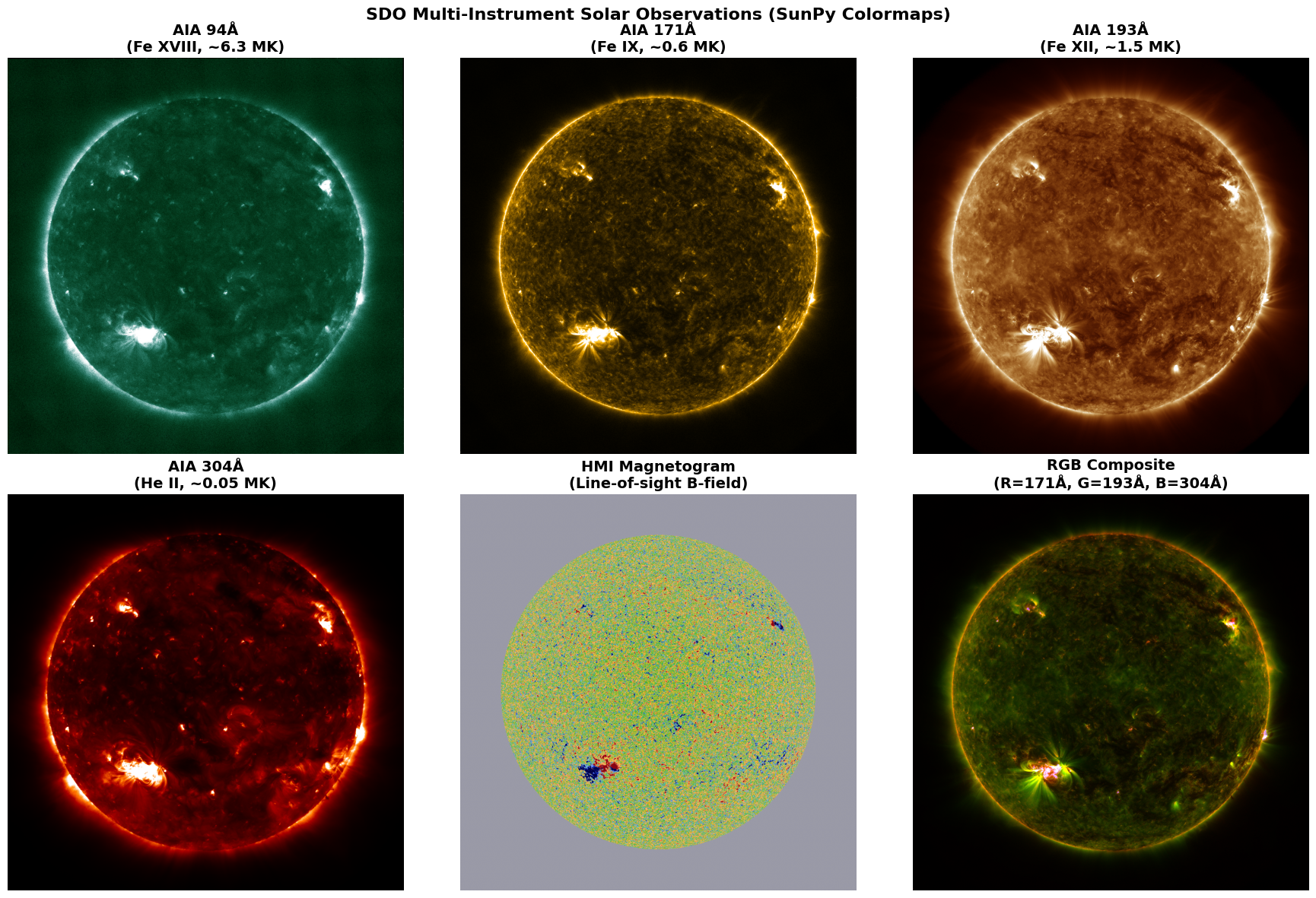
Variables: aia94, aia131, aia171, aia193, aia211, aia304, aia335, aia1600, hmi_m, hmi_bx, hmi_by, hmi_bz, hmi_vAfter loading the NetCDF data, we’ll visualize multiple AIA wavelength channels and HMI magnetic field data to showcase the multi-instrument nature of the SDO dataset.
Professional SunPy Colormaps: This visualization uses the SunPy library’s official SDO colormaps, which are the scientific standard for solar imaging. Each AIA wavelength has a custom colormap designed to highlight features at that temperature regime, and HMI magnetograms use a diverging colormap to show magnetic polarity.
The visualization demonstrates: - AIA channels at different wavelengths (94Å, 171Å, 193Å, 304Å) with proper sdoaia### colormaps - HMI magnetogram displaying magnetic field structure with hmimag colormap - RGB composite combining multiple wavelengths for context - Proper normalization matching professional solar physics standards (1st-99.5th percentile)
import matplotlib.pyplot as plt
import numpy as np
import sunpy.visualization.colormaps as sunpy_cm
import hdf5plugin  # Required to enable HDF5 compression filters
import glob
import json
import xarray as xr

# Load metadata to extract variable information
with open("sdo_geocroissant.json", "r") as f:
    metadata = json.load(f)

# Find NetCDF files
data_dir = metadata['distribution'][0]['contentUrl']
nc_files = sorted(glob.glob(f"{data_dir}/*.nc"))

# Extract variable names from metadata
fields = metadata['recordSet'][0]['field']
aia_vars = [f['name'] for f in fields if 'aia' in f['name']][:4]
hmi_vars = [f['name'] for f in fields if 'hmi' in f['name']][:1]

# Load NetCDF data using xarray with h5netcdf engine
ds = xr.open_dataset(nc_files[0], engine='h5netcdf')
aia94 = ds[aia_vars[0]].values
aia171 = ds[aia_vars[1]].values
aia193 = ds[aia_vars[2]].values
aia304 = ds[aia_vars[3]].values
hmi_m = ds[hmi_vars[0]].values
ds.close()

# Create visualization with proper SunPy colormaps
fig, axes = plt.subplots(2, 3, figsize=(18, 12))

def display_channel(ax, data, title, colormap_name):
    """Display a channel with proper SunPy colormap normalization"""
    # Calculate normalization range
    vmin = np.percentile(data[np.isfinite(data)], 1)
    vmax = np.percentile(data[np.isfinite(data)], 99.5)

    # Normalize data to [0, 1] range
    normalized = np.clip((data - vmin) / (vmax - vmin), 0, 1)

    # Apply SunPy colormap
    cmap = sunpy_cm.cmlist[colormap_name]
    colored_data = cmap(normalized[::-1])  # Flip vertically for proper orientation

    im = ax.imshow(colored_data, origin='lower')
    ax.set_title(title, fontsize=14, fontweight='bold')
    ax.axis('off')

# Display AIA EUV channels with proper SunPy colormaps
display_channel(axes[0, 0], aia94, 'AIA 94Å\n(Fe XVIII, ~6.3 MK)', 'sdoaia94')
display_channel(axes[0, 1], aia171, 'AIA 171Å\n(Fe IX, ~0.6 MK)', 'sdoaia171')
display_channel(axes[0, 2], aia193, 'AIA 193Å\n(Fe XII, ~1.5 MK)', 'sdoaia193')
display_channel(axes[1, 0], aia304, 'AIA 304Å\n(He II, ~0.05 MK)', 'sdoaia304')

# Display HMI magnetogram with proper symmetric colormap
vmax_mag = np.percentile(np.abs(hmi_m[np.isfinite(hmi_m)]), 99)
normalized_mag = np.clip((hmi_m + vmax_mag) / (2 * vmax_mag), 0, 1)
cmap_mag = sunpy_cm.cmlist['hmimag']
colored_mag = cmap_mag(normalized_mag[::-1])

axes[1, 1].imshow(colored_mag, origin='lower')
axes[1, 1].set_title('HMI Magnetogram\n(Line-of-sight B-field)', fontsize=14, fontweight='bold')
axes[1, 1].axis('off')

# Create RGB composite using normalized SunPy colormap outputs
def normalize_for_rgb(data):
    """Normalize data for RGB composite creation"""
    vmin = np.percentile(data[np.isfinite(data)], 1)
    vmax = np.percentile(data[np.isfinite(data)], 99.9)
    return np.clip((data - vmin) / (vmax - vmin), 0, 1)

# Apply SunPy colormaps and extract RGB channels
aia171_colored = sunpy_cm.cmlist['sdoaia171'](normalize_for_rgb(aia171))
aia193_colored = sunpy_cm.cmlist['sdoaia193'](normalize_for_rgb(aia193))
aia304_colored = sunpy_cm.cmlist['sdoaia304'](normalize_for_rgb(aia304))

# Combine into RGB composite (using luminance from each colored channel)
rgb = np.zeros((*aia171.shape, 3))
rgb[:, :, 0] = aia171_colored[:, :, 0]  # Red channel from 171Å
rgb[:, :, 1] = aia193_colored[:, :, 1]  # Green channel from 193Å
rgb[:, :, 2] = aia304_colored[:, :, 2]  # Blue channel from 304Å

axes[1, 2].imshow(rgb[::-1], origin='lower')
axes[1, 2].set_title('RGB Composite\n(R=171Å, G=193Å, B=304Å)', fontsize=14, fontweight='bold')
axes[1, 2].axis('off')

plt.suptitle('SDO Multi-Instrument Solar Observations (SunPy Colormaps)',
             fontsize=16, fontweight='bold', y=0.98)
plt.tight_layout()
plt.show()