# Install mlcroissant
!pip install -q mlcroissant
[notice] A new release of pip is available: 26.0 -> 26.0.1
[notice] To update, run: pip install --upgrade pipGeocroissant 🥐
Croissant 🥐 is a high-level format for machine learning datasets that combines metadata, resource file descriptions, data structure, and default ML semantics into a single file.
Croissant builds on schema.org, and its sc:Dataset vocabulary, a widely used format to represent datasets on the Web, and make them searchable.
GeoCroissant extends Croissant with geospatial concepts (e.g., spatial extents, coordinate reference systems, temporal coverage), enabling rich, location-aware metadata for Earth-observation and other spatial datasets.
The mlcroissant Python library empowers developers to interact with Croissant:
# Install mlcroissant
!pip install -q mlcroissant
[notice] A new release of pip is available: 26.0 -> 26.0.1
[notice] To update, run: pip install --upgrade pipLet’s try a concrete example with the HLS Burn Scars dataset hosted on Hugging Face.
In this tutorial, we’ll programmatically generate the Croissant JSON-LD metadata for the dataset using the mlcroissant Python package.
Finally, we’ll validate and inspect the metadata structure.
import json
from datetime import datetime

# Create a proper GeoCroissant JSON-LD document according to the schema
geocroissant_json = {
    "@context": {
        "@language": "en",
        "@vocab": "https://schema.org/",
        "citeAs": "cr:citeAs",
        "column": "cr:column",
        "conformsTo": "dct:conformsTo",
        "cr": "http://mlcommons.org/croissant/",
        "geocr": "http://mlcommons.org/croissant/geo/",
        "rai": "http://mlcommons.org/croissant/RAI/",
        "dct": "http://purl.org/dc/terms/",
        "sc": "https://schema.org/",
        "data": {
            "@id": "cr:data",
            "@type": "@json"
        },
        "examples": {
            "@id": "cr:examples",
            "@type": "@json"
        },
        "dataBiases": "cr:dataBiases",
        "dataCollection": "cr:dataCollection",
        "dataType": {
            "@id": "cr:dataType",
            "@type": "@vocab"
        },
        "extract": "cr:extract",
        "field": "cr:field",
        "fileProperty": "cr:fileProperty",
        "fileObject": "cr:fileObject",
        "fileSet": "cr:fileSet",
        "format": "cr:format",
        "includes": "cr:includes",
        "isLiveDataset": "cr:isLiveDataset",
        "jsonPath": "cr:jsonPath",
        "key": "cr:key",
        "md5": "cr:md5",
        "parentField": "cr:parentField",
        "path": "cr:path",
        "personalSensitiveInformation": "cr:personalSensitiveInformation",
        "recordSet": "cr:recordSet",
        "references": "cr:references",
        "regex": "cr:regex",
        "repeated": "cr:repeated",
        "replace": "cr:replace",
        "samplingRate": "cr:samplingRate",
        "separator": "cr:separator",
        "source": "cr:source",
        "subField": "cr:subField",
        "transform": "cr:transform"
    },
    "@type": "sc:Dataset",
    "name": "hls_burn_scars",
    "description": "Geospatial dataset extracted from local hls_burn_scars directory containing Harmonized Landsat and Sentinel-2 imagery of burn scars and the associated masks.",
    "url": "file://./hls_burn_scars",
    "citeAs": "@dataset{hls_burn_scars, title={hls_burn_scars geospatial dataset}, year={2026}, url={file://./hls_burn_scars}}",
    "datePublished": datetime.now().strftime("%Y-%m-%d"),
    "version": "1.0",
    "license": "Unknown",
    "conformsTo": [
        "http://mlcommons.org/croissant/1.1",
        "http://mlcommons.org/croissant/geo/1.0"
    ],
    "identifier": "10.57967/hf/0956",
    "alternateName": ["ibm-nasa-geospatial/hls_burn_scars"],
    "creator": {
        "@type": "Organization",
        "name": "IBM-NASA Prithvi Models Family",
        "url": "https://huggingface.co/ibm-nasa-geospatial"
    },
    "keywords": [
        "hls_burn_scars",
        "HLS",
        "burn scars",
        "fire",
        "remote sensing",
        "satellite imagery",
        "Landsat",
        "Sentinel-2",
        "geospatial",
        "English",
        "cc-by-4.0",
        "1K - 10K",
        "Image",
        "Datasets",
        "Croissant",
        "doi:10.57967/hf/0956",
        "🇺🇸 Region: US"
    ],
    "temporalCoverage": "2018-01-01/2021-12-31",
    "geocr:temporalResolution": {
        "@type": "QuantitativeValue",
        "value": 8,
        "unitText": "weeks"
    },
    "geocr:coordinateReferenceSystem": "EPSG:32610",
    "spatialCoverage": {
        "@type": "Place",
        "geo": {
            "@type": "GeoShape",
            "box": "32.0 -125.0 42.0 -114.0"
        }
    },
    "geocr:spatialResolution": {
        "@type": "QuantitativeValue",
        "value": 30.0,
        "unitText": "m"
    },
    "geocr:samplingStrategy": "Subsetted to 512x512 pixel windows covering burn scar areas",
    "geocr:spectralBandMetadata": [
        {
            "@type": "geocr:SpectralBand",
            "name": "Blue",
            "geocr:centerWavelength": {
                "@type": "QuantitativeValue",
                "value": 490,
                "unitText": "nm"
            },
            "geocr:bandwidth": {
                "@type": "QuantitativeValue",
                "value": 65,
                "unitText": "nm"
            }
        },
        {
            "@type": "geocr:SpectralBand",
            "name": "Green",
            "geocr:centerWavelength": {
                "@type": "QuantitativeValue",
                "value": 560,
                "unitText": "nm"
            },
            "geocr:bandwidth": {
                "@type": "QuantitativeValue",
                "value": 60,
                "unitText": "nm"
            }
        },
        {
            "@type": "geocr:SpectralBand",
            "name": "Red",
            "geocr:centerWavelength": {
                "@type": "QuantitativeValue",
                "value": 665,
                "unitText": "nm"
            },
            "geocr:bandwidth": {
                "@type": "QuantitativeValue",
                "value": 30,
                "unitText": "nm"
            }
        },
        {
            "@type": "geocr:SpectralBand",
            "name": "NIR",
            "geocr:centerWavelength": {
                "@type": "QuantitativeValue",
                "value": 865,
                "unitText": "nm"
            },
            "geocr:bandwidth": {
                "@type": "QuantitativeValue",
                "value": 30,
                "unitText": "nm"
            }
        },
        {
            "@type": "geocr:SpectralBand",
            "name": "SWIR1",
            "geocr:centerWavelength": {
                "@type": "QuantitativeValue",
                "value": 1610,
                "unitText": "nm"
            },
            "geocr:bandwidth": {
                "@type": "QuantitativeValue",
                "value": 90,
                "unitText": "nm"
            }
        },
        {
            "@type": "geocr:SpectralBand",
            "name": "SWIR2",
            "geocr:centerWavelength": {
                "@type": "QuantitativeValue",
                "value": 2200,
                "unitText": "nm"
            },
            "geocr:bandwidth": {
                "@type": "QuantitativeValue",
                "value": 180,
                "unitText": "nm"
            }
        }
    ],
    "distribution": [
        {
            "@type": "cr:FileObject",
            "@id": "data_repo",
            "name": "data_repo",
            "description": "Directory containing the dataset files",
            "contentUrl": "./hls_burn_scars",
            "encodingFormat": "local_directory",
            "md5": "placeholder_hash_for_directory"
        },
        {
            "@type": "cr:FileSet",
            "@id": "tiff-files",
            "name": "tiff-files",
            "description": "All TIFF files (images and masks).",
            "containedIn": {
                "@id": "data_repo"
            },
            "encodingFormat": "image/tiff",
            "includes": "**/*.tif"
        }
    ],
    "recordSet": [
        {
            "@type": "cr:RecordSet",
            "@id": "hls_burn_scars",
            "name": "hls_burn_scars",
            "description": "hls_burn_scars dataset with satellite imagery and mask annotations.",
            "field": [
                {
                    "@type": "cr:Field",
                    "@id": "hls_burn_scars/image",
                    "name": "hls_burn_scars/image",
                    "description": "File path to satellite imagery with multiple spectral bands converted to reflectance.",
                    "dataType": "sc:Text",
                    "source": {
                        "fileSet": {
                            "@id": "tiff-files"
                        },
                        "extract": {
                            "fileProperty": "fullpath"
                        },
                        "transform": {
                            "regex": ".*_merged\\.tif$"
                        }
                    },
                    "geocr:bandConfiguration": {
                        "@type": "geocr:BandConfiguration",
                        "geocr:totalBands": 6,
                        "geocr:bandNameList": ["Blue", "Green", "Red", "NIR", "SWIR1", "SWIR2"]
                    }
                },
                {
                    "@type": "cr:Field",
                    "@id": "hls_burn_scars/mask",
                    "name": "hls_burn_scars/mask",
                    "description": "File path to mask annotations with values representing different classes.",
                    "dataType": "sc:Text",
                    "source": {
                        "fileSet": {
                            "@id": "tiff-files"
                        },
                        "extract": {
                            "fileProperty": "fullpath"
                        },
                        "transform": {
                            "regex": ".*\\.mask\\.tif$"
                        }
                    },
                    "geocr:bandConfiguration": {
                        "@type": "geocr:BandConfiguration",
                        "geocr:totalBands": 1,
                        "geocr:bandNameList": ["mask"]
                    }
                }
            ]
        }
    ]
}

# Write the GeoCroissant JSON-LD to file
with open("croissant.json", "w") as f:
    json.dump(geocroissant_json, f, indent=2)
When creating Metadata: - We also check for errors in the configuration. - We generate warnings if the configuration doesn’t follow guidelines and best practices.
For instance, in this case:
!mlcroissant validate --jsonld=croissant.jsonI0216 17:12:41.324774 124879480858432 validate.py:53] Done.!pip install -q rasterio
[notice] A new release of pip is available: 26.0 -> 26.0.1
[notice] To update, run: pip install --upgrade pipfrom load_data import load_dataset
import rasterio
import numpy as np
import matplotlib.pyplot as plt
# Load the dataset from the GeoCroissant JSON
dataset = load_dataset(croissant_path="./croissant.json")
# Get the training split
train_ds = dataset["train"]
print(f"Loaded {len(train_ds)} training samples")
print(f"Dataset info: {train_ds.info}")Loaded 540 training samples
Dataset info: {'name': 'hls_burn_scars', 'description': 'Geospatial dataset extracted from local hls_burn_scars directory containing Harmonized Landsat and Sentinel-2 imagery of burn scars and the associated masks.', 'version': '1.0', 'license': 'Unknown', 'spatial_coverage': {'@type': 'Place', 'geo': {'@type': 'GeoShape', 'box': '32.0 -125.0 42.0 -114.0'}}, 'temporal_coverage': '2018-01-01/2021-12-31', 'crs': 'EPSG:32610', 'spatial_resolution': {'@type': 'QuantitativeValue', 'value': 30.0, 'unitText': 'm'}}After loading the dataset, we extract a sample from the training split and visualize both the satellite image and its corresponding burn scar mask.
Key steps:
rasterio.(C, H, W) format to height-width-channel (H, W, C) for visualization.[0,1] range for proper display.matplotlib.# Get a sample
sample = train_ds[0]
# Get the image and mask paths from the sample
image_path = sample["image"]
mask_path = sample["annotation"]
# Read the image and mask files with rasterio
with rasterio.open(image_path) as src_img:
image = src_img.read()
profile = src_img.profile # Keep profile for reference
with rasterio.open(mask_path) as src_mask:
mask = src_mask.read(1)
# Prepare RGB image for visualization
image_rgb = image[:3].transpose(1, 2, 0) # C,H,W to H,W,C
# Normalize each channel separately for display
for i in range(3):
channel = image_rgb[:, :, i]
min_val = np.min(channel)
max_val = np.max(channel)
if max_val > min_val:
image_rgb[:, :, i] = (channel - min_val) / (max_val - min_val)
# Plot image and mask side-by-side
fig, axs = plt.subplots(1, 2, figsize=(12, 6))
axs[0].imshow(image_rgb)
axs[0].set_title("Image (RGB)")
axs[0].axis("off")
axs[1].imshow(mask, cmap="gray", vmin=0, vmax=1)
axs[1].set_title("Annotation (Mask)")
axs[1].axis("off")
plt.tight_layout()
plt.show()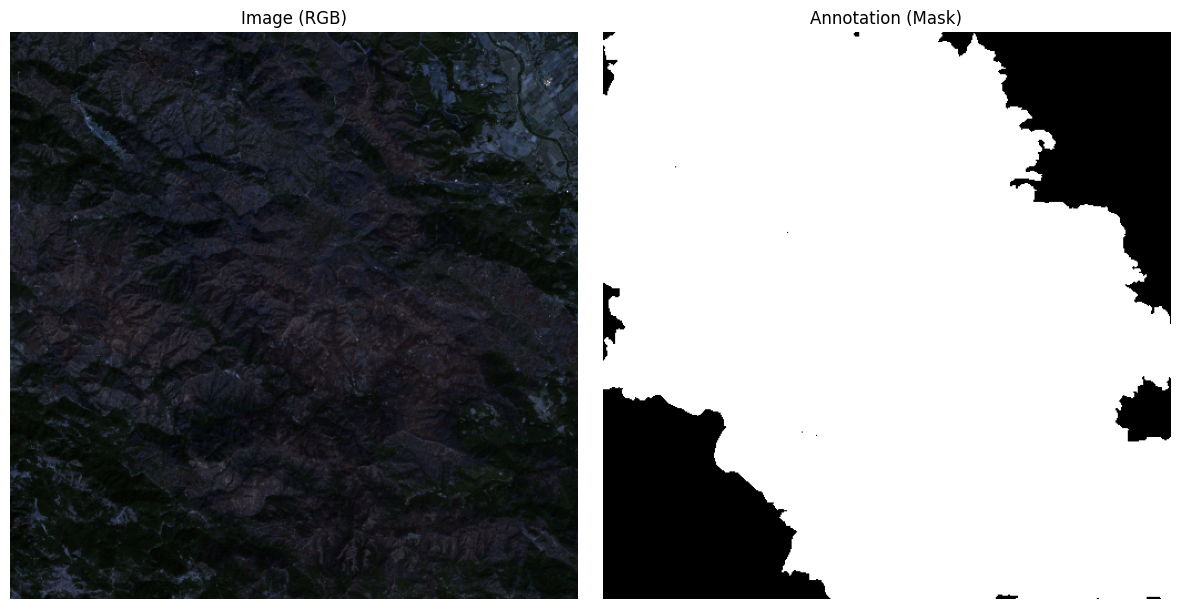
In this notebook, we’ll train a U-Net model:
hls.py that defines the burn scar dataset structure.import json
import torch
import torch.nn as nn
import torch.nn.functional as F
from torch.utils.data import Dataset, DataLoader
import rasterio
import numpy as np
from tqdm import tqdm
# 1. Load the dataset metadata from GeoCroissant JSON
with open("./croissant.json", "r") as f:
croissant_metadata = json.load(f)Loaded 540 training samplesBurnScarsDataset class to load and preprocess .tif satellite images and burn scar masks using rasterio.# 2. Data pipeline
class BurnScarsDataset(Dataset):
def __init__(self, hls_dataset):
self.dataset = hls_dataset
def __len__(self):
return len(self.dataset)
def __getitem__(self, idx):
sample = self.dataset[idx]
with rasterio.open(sample["image"]) as img_file:
image = img_file.read([1, 2, 3])
image = image.astype("float32") / 255.0
image = torch.from_numpy(image).float() # (C, H, W)
with rasterio.open(sample["annotation"]) as mask_file:
mask = mask_file.read(1)
mask = torch.from_numpy(mask).long() # (H, W)
mask = (mask > 0).long() # Ensure binary
return image, mask
batch_size = 8
train_dataset = BurnScarsDataset(train_ds)
train_loader = DataLoader(train_dataset, batch_size=batch_size, shuffle=True, pin_memory=True)# 4. U-Net Model
class DoubleConv(nn.Module):
def __init__(self, in_channels, out_channels):
super().__init__()
self.conv = nn.Sequential(
nn.Conv2d(in_channels, out_channels, kernel_size=3, padding=1),
nn.BatchNorm2d(out_channels),
nn.ReLU(inplace=True),
nn.Conv2d(out_channels, out_channels, kernel_size=3, padding=1),
nn.BatchNorm2d(out_channels),
nn.ReLU(inplace=True)
)
def forward(self, x):
return self.conv(x)
class UNet(nn.Module):
def __init__(self, n_channels=3, n_classes=1):
super().__init__()
self.inc = DoubleConv(n_channels, 64)
self.down1 = nn.Sequential(nn.MaxPool2d(2), DoubleConv(64, 128))
self.down2 = nn.Sequential(nn.MaxPool2d(2), DoubleConv(128, 256))
self.down3 = nn.Sequential(nn.MaxPool2d(2), DoubleConv(256, 512))
self.down4 = nn.Sequential(nn.MaxPool2d(2), DoubleConv(512, 1024))
self.up1 = nn.ConvTranspose2d(1024, 512, kernel_size=2, stride=2)
self.conv1 = DoubleConv(1024, 512)
self.up2 = nn.ConvTranspose2d(512, 256, kernel_size=2, stride=2)
self.conv2 = DoubleConv(512, 256)
self.up3 = nn.ConvTranspose2d(256, 128, kernel_size=2, stride=2)
self.conv3 = DoubleConv(256, 128)
self.up4 = nn.ConvTranspose2d(128, 64, kernel_size=2, stride=2)
self.conv4 = DoubleConv(128, 64)
self.outc = nn.Conv2d(64, n_classes, kernel_size=1)
def forward(self, x):
x1 = self.inc(x)
x2 = self.down1(x1)
x3 = self.down2(x2)
x4 = self.down3(x3)
x5 = self.down4(x4)
x = self.up1(x5)
x = self.conv1(torch.cat([x, x4], dim=1))
x = self.up2(x)
x = self.conv2(torch.cat([x, x3], dim=1))
x = self.up3(x)
x = self.conv3(torch.cat([x, x2], dim=1))
x = self.up4(x)
x = self.conv4(torch.cat([x, x1], dim=1))
logits = self.outc(x)
return logits# 5. Setup device, model, optimizer, loss
device = torch.device("cuda" if torch.cuda.is_available() else "cpu")
print("Using device:", device)
model = UNet(n_channels=3, n_classes=1).to(device)
optimizer = torch.optim.Adam(model.parameters(), lr=1e-3)
criterion = nn.BCEWithLogitsLoss()Using device: cpu# 6. Training
epochs = 5
for epoch in range(1, epochs+1):
model.train()
total_loss = 0.0
loop = tqdm(train_loader, desc=f"Epoch {epoch} [Train]", leave=False)
for images, masks in loop:
images = images.to(device, non_blocking=True)
masks = masks.to(device, non_blocking=True).float()
outputs = model(images)
outputs = outputs.squeeze(1) # (B, H, W)
loss = criterion(outputs, masks)
optimizer.zero_grad()
loss.backward()
optimizer.step()
total_loss += loss.item()
loop.set_postfix(loss=loss.item())
print(f"Epoch {epoch} Train Loss: {total_loss/len(train_loader):.4f}")Epoch 1 Train Loss: 0.3494
Epoch 2 Train Loss: 0.2761
Epoch 3 Train Loss: 0.2591
Epoch 4 Train Loss: 0.2272
Epoch 5 Train Loss: 0.2105# 7. Testing
model.eval()
model = model.to(device)
total_val_loss = 0.0
num_examples = 0
true_positives = 0
with torch.no_grad():
for images, masks in tqdm(train_loader, desc=f"Epoch {epoch} [Val]", leave=False):
images = images.to(device, non_blocking=True)
masks = masks.to(device, non_blocking=True)
outputs = model(images)
outputs = outputs.squeeze(1)
preds = (torch.sigmoid(outputs) > 0.5).long()
total_val_loss += criterion(outputs, masks.float()).item()
true_positives += (preds == masks).sum().item()
num_examples += masks.numel()
val_accuracy = true_positives / num_examples * 100
print(f"Epoch {epoch} Val Loss: {total_val_loss/len(train_loader):.4f} | Accuracy: {val_accuracy:.2f}%")Epoch 5 Val Loss: 0.3564 | Accuracy: 87.56%